PdosPlot

import sisl

# This is just for convenience to retreive files
siesta_files = (
    sisl._environ.get_environ_variable("SISL_FILES_TESTS") / "sisl" / "io" / "siesta"
)

info:0: SislInfo: Please install tqdm (pip install tqdm) for better looking progress bars

We are going to get the PDOS from a SIESTA .PDOS file, but we could get it from some other source, e.g. a hamiltonian.

plot = sisl.get_sile(siesta_files / "SrTiO3.PDOS").plot(Erange=[-10, 10])

By default, a PDOS plot shows the total density of states:

plot

_ipython_canary_method_should_not_exist_ False
_ipython_display_ True

PDOS groups

There’s a very important setting in the PdosPlot: groups. This setting expects a list of orbital groups, where each group is a dictionary that can specify - species - atoms - orbitals (the orbital name) - n, l, m (the quantum numbers) - Z (the Z shell of the orbital) - spin

involved in the PDOS line that you want to draw. Apart from that, a group also accepts the name, color, linewidth and dash keys that manage the aesthetics of the line and reduce, which indicates the method to use for accumulating orbital contributions: "mean" averages over orbitals while "sum" simply accumulates all contributions. Finally, scale lets you multiply the DOS of the group by whatever factor you want.

Here is an example of how to use the groups setting to create a line that displays the Oxygen 2p PDOS:

plot.update_inputs(
    groups=[{"name": "My first PDOS (Oxygen)", "species": ["O"], "n": 2, "l": 1}]
)
# or (it's equivalent)
plot.update_inputs(
    groups=[
        {
            "name": "My first PDOS (Oxygen)",
            "species": ["O"],
            "orbitals": ["2pzZ1", "2pzZ2", "2pxZ1", "2pxZ2", "2pyZ1", "2pyZ2"],
        }
    ]
)

_ipython_canary_method_should_not_exist_ False
_ipython_display_ True

And now we are going to create three lines, one for each species

plot.update_inputs(
    groups=[
        {
            "name": "Oxygen",
            "species": ["O"],
            "color": "darkred",
            "dash": "dash",
            "reduce": "mean",
        },
        {
            "name": "Titanium",
            "species": ["Ti"],
            "color": "gray",
            "size": 3,
            "reduce": "mean",
        },
        {"name": "Sr", "species": ["Sr"], "color": "green", "reduce": "mean"},
    ],
    Erange=[-5, 5],
)

_ipython_canary_method_should_not_exist_ False
_ipython_display_ True

It’s interesting to note that the atoms key of each group accepts the same possibilities as the atoms argument of the Geometry methods. Therefore, you can use indices, categories, dictionaries, strings…

For example:

# Let's import the AtomZ and AtomOdd categories just to play with them
from sisl.geom import AtomZ, AtomOdd

plot.update_inputs(
    groups=[
        {"atoms": [0, 1], "name": "Atoms 0 and 1"},
        {"atoms": {"Z": 8}, "name": "Atoms with Z=8"},
        {"atoms": AtomZ(8) & ~AtomOdd(), "name": "Oxygens with even indices"},
    ]
)

_ipython_canary_method_should_not_exist_ False
_ipython_display_ True

Easy and fast DOS splitting

As you might have noticed, sometimes it might be cumbersome to build all the groups you want. If your needs are simple and you don’t need the flexibility of defining every parameter by yourself, there is a set of methods that will help you explore your PDOS data faster than ever before. These are: split_DOS, split_groups, update_groups, remove_groups and add_groups.

Let’s begin with split_DOS. As you can imagine, this method splits the density of states:

plot.split_DOS()

_ipython_canary_method_should_not_exist_ False
_ipython_display_ True

By default, it splits on the different species, but you can use the on argument to change that.

plot.split_DOS(on="atoms")

_ipython_canary_method_should_not_exist_ False
_ipython_display_ True

Now we have the contribution of each atom.

But here comes the powerful part: split_DOS accepts as keyword arguments all the keys that a group accepts. Then, it adds that extra constrain to the splitting by adding the value to each group. So, if we want to get the separate contributions of all oxygen atoms, we can impose an extra constraint on species:

plot.split_DOS(on="atoms", species=["O"], name="Oxygen $atoms")

_ipython_canary_method_should_not_exist_ False
_ipython_display_ True

and then we have only the oxygen atoms, which are all equivalent.

Note that we also set a name for all groups, with the additional twist that we used the templating supported by split_DOS. If you are splitting on parameter, you can use $parameter inside your name and the method will replace it with the value for each group. In this case parameter was atoms, but it could be anything you are splitting the DOS on.

You can also exclude some values of the parameter you are splitting on:

plot.split_DOS(on="atoms", exclude=[1, 3])

_ipython_canary_method_should_not_exist_ False
_ipython_display_ True

Or indicate the only values that you want:

plot.split_DOS(on="atoms", only=[0, 2])

_ipython_canary_method_should_not_exist_ False
_ipython_display_ True

Finally, if you want to split on multiple parameters at the same time, you can use + between different parameters. For example, to get all the oxygen orbitals:

plot.split_DOS(on="n+l+m", species=["O"], name="Oxygen")

_ipython_canary_method_should_not_exist_ False
_ipython_display_ True

Managing existing groups

Not only you can create groups easily with split_DOS, but it’s also easy to manage the groups that you have created.

The methods that help you accomplish this are split_groups, update_groups, remove_groups. All three methods accept an undefined number of arguments that are used to select the groups you want to act on. You can refer to groups by their name (using a str) or their position (using an int). It’s very easy to understand with examples. Then, keyword arguments depend on the functionality of each method.

For example, let’s say that we have splitted the DOS on species

plot.split_DOS(name="$species")

_ipython_canary_method_should_not_exist_ False
_ipython_display_ True

and we want to remove the Sr and O lines. That’s easy:

plot.remove_groups("Sr", 2)

_ipython_canary_method_should_not_exist_ False
_ipython_display_ True

We have indicated that we wanted to remove the group with name "Sr" and the 2nd group. Simple, isn’t it?

Now that we know how to indicate the groups that we want to act on, let’s use it to get the total Sr contribution, and then the Ti and O contributions splitted by n and l.

It sounds difficult, but it’s actually not. Just split the DOS on species:

plot.split_DOS(name="$species", reduce="mean")

_ipython_canary_method_should_not_exist_ False
_ipython_display_ True

And then use split_groups to split only the groups that we want to split:

plot.split_groups("Sr", 2, on="n+l", dash="dot").show("png")

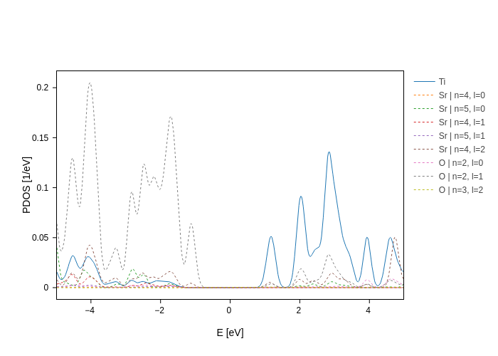
Notice how we’ve also set dash for all the groups that split_groups has generated. We can do this because split_groups works exactly as split_DOS, with the only difference that splits specific groups.

Just as a last thing, we will let you figure out how update_groups works:

plot.update_groups("Ti", color="red", size=4)

_ipython_canary_method_should_not_exist_ False
_ipython_display_ True

We hope you enjoyed what you learned!