import numpy as np
import sisl as si
import matplotlib.pyplot as plt

%matplotlib inline

Anomalous Hall conductivity (AHC) for graphene

This tutorial will describe a complete walk-through of how to calculate the anomalous Hall conductivity for graphene.

Warning

<p>
    This tutorial is not meant for publication ready results.
    Numbers, such as the $k$-point sampling should always be converged before publication is made. The number of $k$-points used here are too small!

Creating the geometry to investigate

Our system of interest will be the pristine graphene system, from a DFT (SIESTA) calculation.

H = si.get_sile("siesta_2/RUN.fdf").read_hamiltonian()

The anomalous Hall conductivity (AHC) requires a rather dense $k$ grid. It is related to the Berry curvature defined as:

$${\mathbf{\Omega }}_{i,\alpha \beta }=2i{\hslash }^2\sum _{j\ne i}\frac{{\hat{v}}_{ij}^{\alpha }{\hat{v}}_{ji}^{\beta }}{[{ϵ}_j-{ϵ}_i{]}^2+i{\eta }^2}$$

where $\hat{v}$ is the velocity operator. One can determine that the units of this quantity is ${\mathrm{Ang}}^2$. The AHC can then be calculated via:

$${\sigma }_{\alpha \beta }=\frac{-e^2}{\hslash }\int \mathrm{d}\mathbf{k}\sum _i{f}_i{\mathrm{\Omega }}_{i,\alpha \beta }(\mathbf{k}).$$

This method is implemented in sisl.physics.electron.ahc. The units of AHC is $\mathrm{S}/{\mathrm{Ang}}^{2-D}$ which for 2D systems is just $\mathrm{S}$.

Its API looks like, hold on, there’s a lot to grasp:

help(si.physics.electron.ahc)

Help on function ahc in module sisl.physics.electron:

ahc(bz: 'BrillouinZone', k_average: 'bool' = True, *, distribution: 'DistributionType' = 'step', eigenstate_kwargs={}, apply_kwargs={}, **berry_kwargs) -> 'np.ndarray'
    Electronic anomalous Hall conductivity for a given `BrillouinZone` integral

    .. math::
       \sigma_{\alpha\beta} = \frac{-e^2}{\hbar}\int\,\mathrm d\mathbf k\sum_i f_i\Omega_{i,\alpha\beta}(\mathbf k)

    where :math:`\Omega_{i,\alpha\beta}` and :math:`f_i` is the Berry curvature and occupation
    for state :math:`i`.

    The conductivity will be averaged by volume of the periodic unit cell.
    Hence the unit of `ahc` depends on the periodic unit cell.
    See `~sisl.Lattice.volumef` for details.

    See :cite:`Wang2006` for details on the implementation.

    Parameters
    ----------
    bz :
        containing the integration grid and has the ``bz.parent`` as an instance of Hamiltonian.
    k_average :
        if `True`, the returned quantity is averaged over `bz`, else all k-point
        contributions will be collected (in the 1st dimension).
        Note, for large `bz` integrations this may explode the memory usage.
    distribution :
        An optional distribution enabling one to automatically sum states
        across occupied/unoccupied states.
    eigenstate_kwargs :
       keyword arguments passed directly to the ``contour.eigenstate`` method.
       One should *not* pass a ``k`` or a ``wrap`` keyword argument as they are
       already used.
    apply_kwargs :
       keyword arguments passed directly to ``bz.apply.renew(**apply_kwargs)``.
    **berry_kwargs :
        arguments passed directly to the `berry_curvature` method.

        Here one can pass `derivative_kwargs` to pass flags to the
        `derivative` method. In particular ``axes`` can be used
        to speedup the calculation (by omitting certain directions).

    Examples
    --------

    To calculate the AHC for a range of energy-points.
    First create ``E`` which is the energy grid.
    In order for the internal algorithm to be able
    to broadcast arrays correctly, we have to allow the eigenvalue
    spectrum to be appended by reshaping.

    >>> E = np.linspace(-2, 2, 51)
    >>> dist = get_distribution("step", x0=E.reshape(-1, 1))
    >>> ahc_cond = ahc(bz, dist)
    >>> assert ahc_cond.shape == (3, 3, len(E))

    Sometimes one wishes to see the k-resolved AHC.
    Be aware that AHC requires a dense k-grid, and hence it might
    require a lot of memory.
    Here it is calculated at :math:`E=0` (default energy reference).

    >>> ahc_cond = ahc(bz, k_average=False)
    >>> assert ahc_cond.shape == (len(bz), 3, 3)

    See Also
    --------
    ~sisl.physics.derivative: method for calculating the exact derivatives
    ~sisl.physics.berry_curvature: method used to calculate the Berry curvature for calculating the conductivity
    ~sisl.Lattice.volumef: volume calculation of the lattice
    shc: spin Hall conductivity

    Returns
    -------
    ahc:
        Anomalous Hall conductivity returned in certain dimensions ``ahc[:, :]``.
        If `sum` is False, it will be at least a 3D array with the 3rd dimension
        having the contribution from state `i`.
        If `k_average` is False, it will have a dimension prepended with
        k-point resolved AHC.
        If one passes `axes` to the `derivative_kwargs` argument one will get
        dimensions according to the number of axes requested, by default all
        axes will be used (even if they are non-periodic).
        The dtype will be imaginary.
        When :math:`D` is the dimensionality of the system we find the unit to be
        :math:`\mathrm S/\mathrm{Ang}^{D-2}`.

---

We will be interested in calculating the ahc for a set of different energies (equivalent to different chemical potentials). So we need to define an energy-range, and a distribution function, here the simple step-function is used.

E = np.linspace(-5, 2, 51)
# When calculating for a variety of energy-points, we have to have an available axis for the eigenvalue distribution
# calculation.
dist = si.get_distribution("step", x0=E.reshape(-1, 1))
# Generally you want a *very* dense k-point grid
bz = si.MonkhorstPack(H, [15, 15, 1], trs=False)

Since we are only interested in the $xy$ plane (there is no periodicity along $z$, hence superfluous calculation), we will try and reduce the computation by specifying which axes we want to calculate the AHC along. Additionally, we can speed up the calculation for matrices that are small, by explicitly specifying them to be calculated in the numpy.ndarray format, as opposed to the default scipy.sparse.csr_matrix format (slower, but much less memory consuming). When dealing with these conductivities it can also be instructive to view the $k$-resolved conductivities at certain energies.

Lastly, eta=True specifies we want to show the progressbar.

ahc = si.physics.electron.ahc(
    bz,
    # yield a k-resolved AHC array
    k_average=False,
    distribution=dist,
    # Speed up by format='array'
    eigenstate_kwargs={"format": "array", "dtype": np.complex128, "eta": True},
    # Speed up by only calculating the xx, xy, yx, yy contributions
    derivative_kwargs={"axes": "xy"},
).real  # we don't need the imaginary part.

MonkhorstPack.ndarray: 100%

 225/225 [00:01<00:00, 208.22k/s]

Now we have a (len(bz), 2, 2, len(E)) AHC array.

plt.plot(E, ahc.sum(0)[0, 1], label=r"$\sigma_{xy}$")
plt.plot(E, ahc.sum(0)[1, 0], label=r"$\sigma_{yx}$")
plt.xlabel("Energy [eV]")
plt.ylabel(r"$\sigma$ [Ang^2]")
plt.legend();

As we can see there are some contributions near $E_F$, and at the lower bands.

The numbers though are not converged, and likely requires more scrutiny (outside the scope of this tutorial).

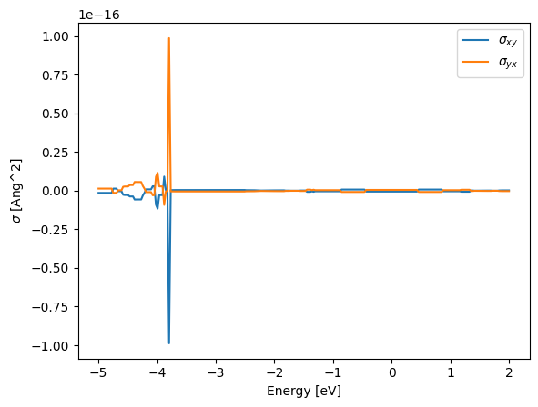
We can now plot the $k$-resolved AHC values at $E_F$:

E0 = np.argmin(np.fabs(E))
kx = np.unique(bz.k[:, 0])
ky = np.unique(bz.k[:, 1])
plt.contourf(
    # unique values along x, y
    kx,
    ky,
    ahc[:, 0, 1, E0].reshape(len(kx), len(ky)),
)
plt.colorbar();

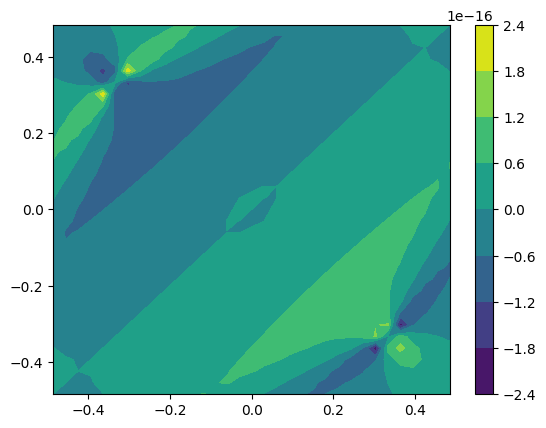
This concludes a simple tutorial on how to calculate the AHC for a given system, and also how to calculate the $k$-resolved AHC.