[1]:
import sisl as si
import numpy as np

%matplotlib inline
import matplotlib.pyplot as plt
Defining orbitals
Orbitals, and basis sets, is a complicated matter that requires a broader set of classes. sisl enables one to use orbitals without information, but also other specialized orbitals, such as atomic orbitals and Gaussian/Slater type orbitals. Information about the different orbitals can be found here.
In this tutorial we will show how one can create different orbitals, and use them.
[2]:
orb = si.Orbital(1.2, q0=1)
print(orb)
Orbital{R: 1.20000, q0: 1.0}
Geometry objects to estimate which atoms interacts with other atoms, and as such they are the back-bone of tight-binding models.Orbitals with spherical shapes
sisl.Here we define the orbital range as the maximum R such that integral:
contains \(99\%\) of the function.
[3]:
r = np.linspace(0, 3, 200)
f = np.exp(-2 * r**2)
sorb = si.SphericalOrbital(1, (r, f), R={"contains": 0.99})
print(sorb)
SphericalOrbital{l: 1, R: 1.2879999999999991, q0: 0.0}
Now we have a spherical orbital with \(l=1\) quantum number. Lets plot its spherical form and its wavefunction:
[4]:
for m in (0, 1):
    # Plotting for theta = phi = 45 angles
    plt.plot(r, sorb.psi_spher(r, 45, 45, m=m), label=f"m={m}")
plt.legend();
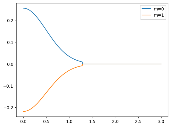
Note how the wavefunction gets truncated at the orbital radius, based on the truncation optimization.
The SphericalOrbital is typically just a temporary orbital array used for creating proper atomic orbitals. Atomic orbitals contains relevant quantum numbers, but also a spherical function. The AtomicOrbital accepts many other possibilities of arguments, please refer to its documentation for detailed explanations.
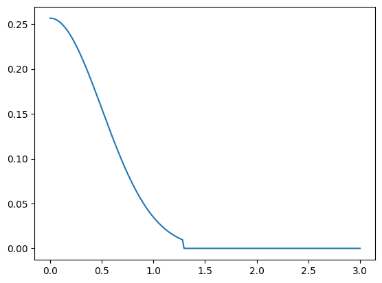
[5]:
aorb = si.AtomicOrbital("pz", spherical=sorb)
plt.plot(r, aorb.psi_spher(r, 45, 45));
Atoms with orbitals
Atoms are defined with 1 or more orbitals. To create an atom with a specific set of orbitals simply do:
[6]:
C = si.Atom(6, [sorb, aorb])
print(C)
Atom{C, Z: 6, mass(au): 12.01070, maxR: 1.28800,
 SphericalOrbital{l: 1, R: 1.2879999999999991, q0: 0.0},
 AtomicOrbital{2pzZ1, q0: 0.0, SphericalOrbital{l: 1, R: 1.2879999999999991, q0: 0.0}}
}
This atom can then further be used in Geometry creations.