First steps
[1]:
import sisl

# We define the root directory where our files are
siesta_files = (
    sisl._environ.get_environ_variable("SISL_FILES_TESTS") / "sisl" / "io" / "siesta"
)
info:0: SislInfo: Please install tqdm (pip install tqdm) for better looking progress bars
Your first plots
The most straightforward way to plot things in sisl is to call their plot method. For example if we have the path to a bands file we can call plot:
[2]:
sisl.get_sile(siesta_files / "SrTiO3.bands").plot()
_ipython_canary_method_should_not_exist_ False
_ipython_display_ True
You can pass arguments to the plotting function:
[3]:
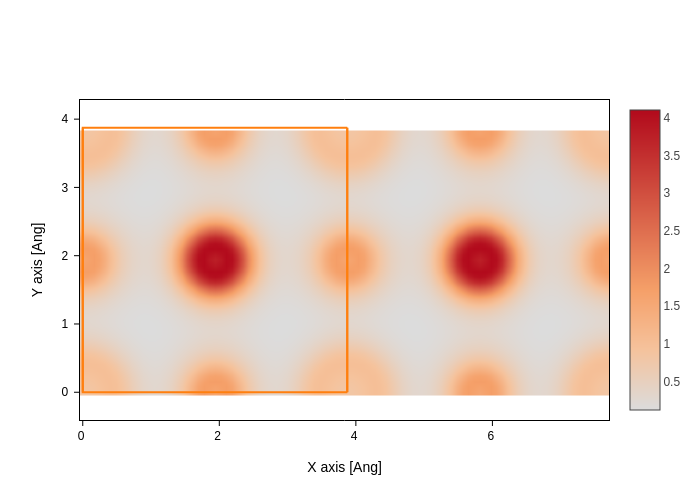
rho_file = sisl.get_sile(siesta_files / "SrTiO3.RHO")
rho_file.plot(axes="xy", nsc=[2, 1, 1], smooth=True).show("png")
Some objects can be plotted in different ways, and just calling plot will do it in the default way. You can however choose which plot you want from the available representations. For example, out of a PDOS file you can plot the PDOS (the default):
[4]:
pdos_file = sisl.get_sile(siesta_files / "SrTiO3.PDOS")

pdos_file.plot(groups=[{"species": "O", "name": "O"}, {"species": "Ti", "name": "Ti"}])
_ipython_canary_method_should_not_exist_ False
_ipython_display_ True
or the geometry (not the default, you need to specify it):
[5]:
pdos_file.plot.geometry(atoms_scale=0.7)
_ipython_canary_method_should_not_exist_ False
_ipython_display_ True
Updating your plots
When you call .plot(), you receive a Plot object:
[6]:
pdos_plot = pdos_file.plot()
type(pdos_plot)
[6]:
sisl.viz.plots.pdos.PdosPlot
Plot objects are a kind of Workflow. You can check the sisl.nodes documentation to understand what exactly this means. But long story short, this means that the computation is split in multiple nodes, as you can see in the following diagram:
[7]:
pdos_plot.network.visualize(notebook=True)
/opt/hostedtoolcache/Python/3.12.3/x64/lib/python3.12/site-packages/IPython/core/display.py:431: UserWarning:

Consider using IPython.display.IFrame instead
With that knowledge, when you update the inputs of a plot, only the necessary parts are recalculated. In that way, you may avoid repeating expensive calculations or reading to files that no longer exist. Inputs are updated with update_inputs:
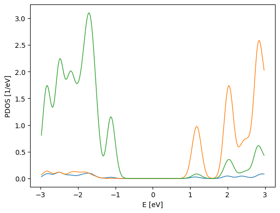
[8]:
pdos_plot.update_inputs(Erange=[-3, 3])
_ipython_canary_method_should_not_exist_ False
_ipython_display_ True
Some inputs are a bit cumbersome to write by hand, and therefore along your journey you’ll find that plots have some helper methods to modify inputs much faster. For example, PdosPlot has the split_DOS method, which generates groups of orbitals for you.
[9]:
pdos_plot.split_DOS()
_ipython_canary_method_should_not_exist_ False
_ipython_display_ True
Don’t worry!
Each plot class has its own dedicated notebook in the documentation to guide you through all the knobs that they have!
Different plotting backends
Hidden between all the inputs, you can find a very special input: backend.
This input allows you to choose the plotting backend used to display a plot. If you don’t like the default one, just change it!
[10]:
pdos_plot.update_inputs(backend="matplotlib")
[10]:
<sisl.viz.plots.pdos.PdosPlot at 0x7fe77f8e22a0>
Let’s go back to the default one, plotly.
[11]:
pdos_plot.update_inputs(backend="plotly")
_ipython_canary_method_should_not_exist_ False
_ipython_display_ True
Further customization
If you are a master of some backend, you’ll be happy to know that you can run any backend specific method on the plot. For example, plotly has a method called add_vline that draws a vertical line:
[12]:
pdos_plot.add_vline(-1).add_vline(2)
add_vline True
In fact, if you need the raw figure for something, you can find it under the figure attribute.
[13]:
type(pdos_plot.figure)
[13]:
plotly.graph_objs._figure.Figure
Discover more
This notebook has shown you the most basic features of the framework with the hope that you will be hooked into it :)
If it succeeded, we invite you to check the rest of the documentation. It only gets better from here!